LeetGPU Challenge #2: Matrix Multiplication (Triton)

It’s been a few days since the first blog post. I got a bit distracted trying to add comment functionality to this website and it took way longer than expected lol. I’ve been solving a lot of LeetGPU challenges in the meantime as well though! It’s fun and very hard to stop so the blog posts are gonna lag behind by quite a lot 😆.

Anyways, I really enjoyed solving the challenge for day 2. It had a massive jump in difficulty from the last one imo and the solution involved some optimizations that were interesting to learn about and keep in mind for the future.

The Challenge: Matrix Multiplication

The task is to multiply two matrices. Given matrix A of dimensions MxN and matrix B of dimensions NxK, we need to compute the product matrix C = A x B, which will have dimensions MxK. All matrices are stored in row-major format.

Constraints:

• 1 ≤ M, N, K ≤ 8192
• Performance is measured with M = 8192, N = 6144, K = 4096

Example

1
Input:  A (2x2) = [[1.0, 2.0], [3.0, 4.0]]
2
        B (2x2) = [[5.0, 6.0], [7.0, 8.0]]
3
Output: C (2x2) = [[19.0, 22.0], [43.0, 50.0]]

Here’s how we would solve this simply on the CPU:

1
M = N = K = 2
2
A = [[1.0, 2.0], [3.0, 4.0]]
3
B = [[5.0, 6.0], [7.0, 8.0]]
4
C = []
5
for m in range(M):
6
    C.append([]) # Initialize empty row on output
7
    for k in range(K):
8
        sum = 0.0
9
        for n in range(N):
10
            sum += A[m][n] * B[n][k]
11
        C[m].append(sum)
12
# C now contains [[19.0, 22.0], [43.0, 50.0]]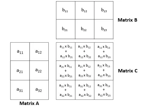

It basically does the following:

1. Read A’s rows one by one (Row length: N) m in range(M)
2. Read B’s columns one by one (Column length: N) k in range(K)
3. For each element in the row x column pair, calculate row[n] * col[n] and accumulate the result in C[m][k] through summation n in range(N)

Solving the Challenge

Initially I thought this would be pretty easy to solve. Just parallelize the loops and we’re good to go. But as I was writing the code I realized the naive way I was trying to solve it left a lot of performance on the table.

I think it’s a good starting point though and it’s good to see some bad examples too so we know what to avoid so let’s go through the naive solution first, pinpoint the parts that make it bad and then we can talk about the optimizations that turn it into the perfect kernel :)

Here’s the pseudocode for the naive solution:

1
def matrix_multiply_gpu(A, B, C, M, N, K):
2
    # We need to parallelize the 3 loops
3
    BLOCK_SIZE_M = 2 # for rows of A (A is MxN -> M for rows)
4
    BLOCK_SIZE_K = 2 # for cols of B (B is NxK -> K for cols)
5
    BLOCK_SIZE_N = 2 # for elements in rows/cols (N for elements)
6

7
    # Calculate the chunks we need to work on
8
    num_blocks_m = ceil(M / BLOCK_SIZE_M)
9
    num_blocks_k = ceil(K / BLOCK_SIZE_K)
10
    num_blocks_n = ceil(N / BLOCK_SIZE_N)
11

12
    # Do a 3 dimensional grid
13
    gpu_programs = get_gpu_programs(
14
        x_id=num_blocks_m, # x for calculating offset into A's rows
15
        y_id=num_blocks_k, # y for calculating offset into B's cols
16
        z_id=num_blocks_n, # z for calculating offset into row/col elements
17
    )
18

19
    # Read rows of A and cols of B
20
    gpu_programs.load_rows(
21
        from=A, offset=x_id * BLOCK_SIZE_M, count=BLOCK_SIZE_M, as=a_rows
22
    )
23
    gpu_programs.load_cols(
24
        from=B, offset=y_id * BLOCK_SIZE_K, count=BLOCK_SIZE_K, as=b_rows
25
    )
26

27
    # Read elements from the loaded rows and cols
28
    gpu_programs.load_elements(
29
        from=a_rows, offset=z_id * BLOCK_SIZE_N, count=BLOCK_SIZE_N, as=row_elements
30
    )
31
    gpu_programs.load_elements(
32
        from=b_cols, offset=z_id * BLOCK_SIZE_N, count=BLOCK_SIZE_N, as=col_elements
33
    )
34

35
    # Calculate the dot product of the loaded elements
36
    gpu_programs.dot_product(
37
        row_elements, col_elements, as=intermediate_result
38
    )
39

40
    # We need to do accumulation since we're processing data in blocks
41
    # So we must read and then add and write
42
    gpu_programs.load_values(
43
        from=C,
44
        rows=x_id * BLOCK_SIZE_M,
45
        cols=y_id * BLOCK_SIZE_K,
46
        as=c_values
47
    )
48
    gpu_programs.store_values(
49
        into=C,
50
        values=c_values + intermediate_result,
51
        at_rows=x_id * BLOCK_SIZE_M,
52
        at_cols=y_id * BLOCK_SIZE_K,
53
    )
54

55
# C is preallocated for us
56
def main(A, B, C, M, N, K):
57
    matrix_multiply_gpu(A, B, C, M, N, K)

The main issues:

• RACE CONDITION (CRITICAL BUG, POTENTIAL FOR WRONG OUTPUT): Keeping in mind that multiple programs execute in parallel, we can see that the part at the end where we try to read from C, add to it, and then store it again (accumulation) is going to fail since multiple programs will try to read and write to it at the same time leading to overwrites and not actual accumulation.
• Efficiency (OPTIMIZATION): Relating to the output again. Accumulating into a GLOBAL location in GPU memory (Where C is) is slow. The intuition you must have to write fast kernels is that you must try to minimize the amount of loads and writes from and into the GLOBAL memory space of the GPU.

The race condition is actually possible to solve by using atomics. Atomics basically give us a way to do operations in a thread safe manner because they combine the read -> modify -> write steps into a single hardware level operation that happens at once atomically. To fix this part in Triton we can use the atomic_add function.

Even with that though we still haven’t solved the efficiency problem AND if we use atomic_add it will make that efficiency problem even worse. Atomics aren’t inherently slow but because there might be a lot of atomic_add operations being done in parallel for the exact same memory spot, there’s a chance for high contention. The atomic operations will basically have to wait for other atomic operations to finish so they can get the latest value in the memory location.

So how do we solve this? Thankfully Triton’s docs just like the first challenge have a tutorial for this exact problem! Official Triton Tutorial on Matrix Multiplication. And as it turns out, there’s a way to do this without atomics and with no risk of race conditions, while also limiting the amount of loads and writes to global memory 🤯. The key idea is tiling combined with local accumulators.

Instead of parallelizing all three loops (for M, K, and N) globally across programs like in our naive solution, we:

1. Parallelize only M and K globally (rows and columns of the output C) so each program handles one tile of the output
2. Move the loop over N inside each program so each program iterates over N sequentially in chunks
3. Use a local accumulator variable to accumulate results as we iterate over N chunks
4. Only write to global memory once at the very end with the final result This way, each program computes one tile of the output matrix independently, so there’s no race condition. And since we’re doing all the accumulation in local variables, we avoid the slow global memory access until the very end.

The approach uses some really important optimization concepts that we should really keep in mind and develop an intuition for not only for matrix multiplication but for any sort of GPU programming that we do. We’ll go through them in deeper detail in the optimizations section below.

Before we do that though let’s take a look at the final pseudocode:

1
def matrix_multiply_gpu(A, B, C, M, N, K):
2
    # We parallelize M and K GLOBALLY (rows and cols of output C)
3
    # So each program handles one tile of the output (C is MxK)
4
    # We still break N into chunks but we iterate over it LOCALLY inside each program
5
    BLOCK_SIZE_M = 64  # for rows of C (And A since they both have M rows)
6
    BLOCK_SIZE_K = 64 # for cols of C (And B since they both have K cols)
7
    BLOCK_SIZE_N = 64  # Chunk size for the local loop over N elements in rows/cols
8

9
    # Calculate the chunks we need to work on
10
    num_blocks_m = ceil(M / BLOCK_SIZE_M)
11
    num_blocks_k = ceil(K / BLOCK_SIZE_K)
12

13
    # Do a 2 dimensional grid
14
    gpu_programs = get_gpu_programs(
15
        x_id=num_blocks_m, # x for calculating offset into C and A's rows
16
        y_id=num_blocks_k, # y for calculating offset into C and B's cols
17
    )
18

19
    # Inside each program allocate an accumulator in on-chip memory
20
    gpu_programs.allocate_local_memory(
21
        rows=BLOCK_SIZE_M,
22
        cols=BLOCK_SIZE_K,
23
        initial_values=0,
24
        as=local_accumulator,
25
    )
26

27
    # Loop over the N elements of rows of A and cols of B in chunks in each program
28
    num_chunks_n = ceil(N / BLOCK_SIZE_N)
29
    for n_chunk in range(num_chunks_n):
30
        # Load BLOCK_SIZE_N elements from BLOCK_SIZE_M rows of A
31
        # Threads within each program work in parallel to load the elements
32
        gpu_programs.load_row_elements(
33
            from=A,
34
            row_offset=x_id * BLOCK_SIZE_M,
35
            row_count=BLOCK_SIZE_M,
36
            element_offset_in_row=n_chunk * BLOCK_SIZE_N,
37
            element_count=BLOCK_SIZE_N,
38
            as=a_elements
39
        )
40

41
        # Load BLOCK_SIZE_N elements from BLOCK_SIZE_K cols of B
42
        # Threads within each program work in parallel to load the elements
43
        gpu_programs.load_col_elements(
44
            from=B,
45
            col_offset=y_id * BLOCK_SIZE_K,
46
            col_count=BLOCK_SIZE_K,
47
            element_offset_in_col=n_chunk * BLOCK_SIZE_N,
48
            element_count=BLOCK_SIZE_N,
49
            as=b_elements
50
        )
51

52
        # Calculate the dot product of the loaded elements
53
        gpu_programs.dot_product(
54
            a_elements, b_elements, as=intermediate_result
55
        )
56

57
        # Add the result to the local accumulator
58
        # It's all in local memory, no contention, no race condition and no slow global memory read and write!!
59
        gpu_programs.add(local_accumulator, intermediate_result, as=local_accumulator)
60

61
    # After the loop, accumulator contains the final result for this tile
62
    # Now we write it to C ONCE (Just one global memory write per result)
63
    gpu_programs.store_values(
64
        into=C,
65
        values=local_accumulator,
66
        at_rows=x_id * BLOCK_SIZE_M,
67
        at_cols=y_id * BLOCK_SIZE_K,
68
    )
69

70
# C is preallocated for us
71
def main(A, B, C, M, N, K):
72
    matrix_multiply_gpu(A, B, C, M, N, K)

Optimizations

Now let’s finally get into all the optimizations that are involved in the pseudocode we just saw that make it so efficient and develop an intuition for them so we can apply them anytime we do GPU programming.

Row-Major Ordering vs Grouped Ordering

When solving this problem a naive solution would be to have each program compute one entire row of the output matrix C. Let’s see what that would look like:

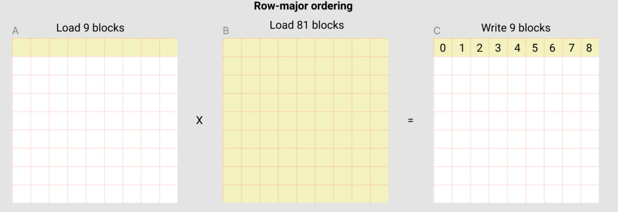
In this row-major ordering approach, each program would:

• Load one row from A (9 blocks in this example)
• Load the entire B matrix (81 blocks in this example)
• Compute one row of C and write it back (9 blocks)
• 90 loads -> 9 results

The issue:

• Every single program needs to load the entire B matrix. If we have 1000 programs computing 1000 rows, we’re loading all of B 1000 times!

We can do much better by using grouped ordering. We basically organize programs into groups that would each work on adjacent tiles in the output C:

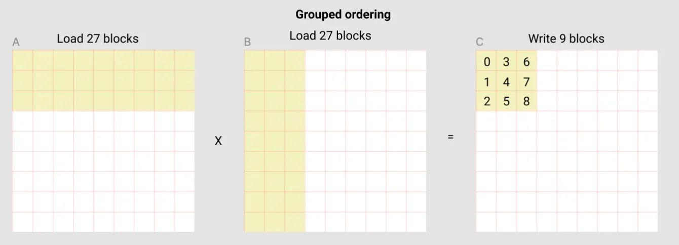
In this approach:

• We divide programs into groups that work to compute adjacent tiles in the output C
  • Imagine 3 programs each working on 3x3 tiles (Like the tile in the image above) starting from top left (the tile being shown) to top right.
  • The tiles these programs work on being adjacent is important for benefiting from the GPU’s memory cache! More on this later.
• Each program loads a tile from A (For 3 rows that’s 27 blocks in total)
• Each program loads a tile from B (For 3 columns that’s 27 blocks in total)
• Each program computes a 3x3 tile of C (9 blocks total)
• 54 loads -> 9 results
  • Combining the 3 programs that we grouped together:
  • Same 3 rows of A being loaded 3 times (27 blocks * 3 programs = 81 blocks total, but cache helps since they’re the same rows!)
  • All columns of B being loaded across the 3 programs (27 blocks per program * 3 programs = 81 blocks total, which is all of B)
  • In total: 81 loads from A + 81 loads from B = 162 loads
  • 162 loads -> 27 results are MUCH better than 90 loads -> 9 results (specially considering that we also benefit from the cache)

This improves 2 things:

• Less Global Memory Reads: We’re loading much less data from the global memory for calculating the same amount of results.
• Cache Utilization: Since we make the programs in the same group work on adjacent tiles, they end up trying to load overlapping or nearby data in the global memory. This means a lot of the times the data might already be in the GPU’s cache for faster access than a normal direct read from the memory.

Local Accumulators

Another optimization being done is the local accumulation technique. Instead of reading from C, modifying it, and writing back (which causes race conditions and is slow), we use a local accumulator. Instead of relying on the global GPU memory for temporary results, we utilize the fast on-chip memory and only write to the global memory at the end ONCE.

This helps us:

• Avoid Race Conditions: Each program has its own accumulator, so there’s no need to read and write into the same global memory location.
• Achieve Better Performance: We’re doing all the work in fast on-chip memory and only touching the slow global memory once at the very end.

The Solution

It’s finally time for the actual implementation and the solution code! As we saw in the previous post, LeetGPU provides us with some boilerplate to get started. Here’s what they give us:

1
import torch
2
import triton
3
import triton.language as tl
4

5
@triton.jit
6
def matrix_multiplication_kernel(
7
    a, b, c, M, N, K, stride_am, stride_an, stride_bn, stride_bk, stride_cm, stride_ck
8
):
9
    pass
10

11
# a, b, c are tensors on the GPU
12
def solve(a: torch.Tensor, b: torch.Tensor, c: torch.Tensor, M: int, N: int, K: int):
13
    stride_am, stride_an = N, 1
14
    stride_bn, stride_bk = K, 1
15
    stride_cm, stride_ck = K, 1
16

17
    grid = (M, K)
18
    matrix_multiplication_kernel[grid](
19
        a, b, c, M, N, K, stride_am, stride_an, stride_bn, stride_bk, stride_cm, stride_ck
20
    )

You’ll notice as you see the solution code below that it looks a bit different from the provided boilerplate because I don’t use the stride parameters that LeetGPU provides. It’s just a personal preference! I prefer to code those explicitly so I can calculate in my head what’s going on better and learn better without relying on helpers.

Another thing you’ll notice is that despite having said “When working on multi dimensional problems we can launch Triton programs using a grid with multiple dimensions so each program can have X, Y, Z… IDs” in the first blog post, in this solution we launch a one dimensional grid and calculate the X, Y IDs manually.

We could definitely use a 2d grid! But if you remember from the optimization section above, we talked about needing to “group” multiple programs together and have them work on adjacent tiles. By default when you launch a grid with multiple dimensions, there’s no guarantee that program with ID=(0,0) is going to be working on data adjacent to program with ID=(0,1) and so on. So we’ll lose the benefit of cache hits. There is a way to map the program_id in that case to a “logical” id that puts (0, 0) and (0, 1) adjacent to each other using some math that a function called swizzle2d in Triton can do for us. But I figured it’s better to explicitly calculate the ID since this is a tutorial and I want to learn and help you guys learn as well. Not to mention the tutorial in Triton’s official docs does the same!

Step 1. Boilerplate

Let’s start with the setup. As we saw before, LeetGPU provides the basic structure, but we’ll customize it for our needs:

1
import torch
2
import triton
3
import triton.language as tl
4

5
@triton.jit
6
def matrix_multiplication_kernel(
7
    a, b, c,
8
    M, N, K,
9
    BLOCK_M: tl.constexpr,
10
    BLOCK_N: tl.constexpr,
11
    BLOCK_K: tl.constexpr,
12
    GROUP_SIZE: tl.constexpr
13
):
14
    pass
15

16
# a, b, c are tensors on the GPU
17
def solve(a: torch.Tensor, b: torch.Tensor, c: torch.Tensor, M: int, N: int, K: int):
18
    BLOCK_M = 64
19
    BLOCK_N = 32
20
    BLOCK_K = 128
21
    GROUP_SIZE = 4
22

23
    grid = (triton.cdiv(M, BLOCK_M) * triton.cdiv(K, BLOCK_K), )
24

25
    matrix_multiplication_kernel[grid](
26
        a, b, c,
27
        M, N, K,
28
        BLOCK_M=BLOCK_M,
29
        BLOCK_N=BLOCK_N,
30
        BLOCK_K=BLOCK_K,
31
        GROUP_SIZE=GROUP_SIZE
32
    )

From the top in solve:

• BLOCK_M, BLOCK_N, and BLOCK_K define the tile sizes we want to work with.
  • BLOCK_M is the amount of rows we want to handle from A and C per program
  • BLOCK_N is the amount of columns we want to handle from A, and the amount of rows we want to handle from B per program (the shared N that they both have)
  • BLOCK_K is the amount of columns we want to handle from B and C per program
  • Notice these aren’t all the same size (64, 32, 128). I did some experimentation and chose the values that gave the best performance for the specific sizes LeetGPU was benchmarking the solution against and the GPU it was running on.
• GROUP_SIZE is how many programs we want to group together. Programs in the same group work on adjacent tiles to help with cache hits.
• The grid size is triton.cdiv(M, BLOCK_M) * triton.cdiv(K, BLOCK_K). This gives us the total number of tiles we need to compute. Again as I said above, we’re using a 1D grid and we’ll manually calculate the X, Y IDs for each program.

Step 2. Calculating the X, Y ID of Programs for Grouped Adjacency

Now we need to figure out which tile each program should work on. Remember that with grouped ordering we need to organize programs into groups that work on adjacent tiles.

1
@triton.jit
2
def matrix_multiplication_kernel(
3
    a, b, c,
4
    M, N, K,
5
    BLOCK_M: tl.constexpr,
6
    BLOCK_N: tl.constexpr,
7
    BLOCK_K: tl.constexpr,
8
    GROUP_SIZE: tl.constexpr
9
):
10
    pid = tl.program_id(axis=0)
11

12
    num_pid_m = tl.cdiv(M, BLOCK_M)
13
    num_pid_k = tl.cdiv(K, BLOCK_K)
14
    num_pid_in_group = GROUP_SIZE * num_pid_k
15

16
    group_id = pid // num_pid_in_group
17
    first_pid_m = group_id * GROUP_SIZE
18
    group_size = tl.minimum(num_pid_m - first_pid_m, GROUP_SIZE)
19

20
    pid_m = first_pid_m + ((pid % num_pid_in_group) % group_size)
21
    pid_k = (pid % num_pid_in_group) // group_size

From the top:

• pid = tl.program_id(axis=0) gets our program ID from the 1D grid.
• num_pid_m = tl.cdiv(M, BLOCK_M) calculates how many tile rows we need (How many chunks of size BLOCK_M fit in M).
• num_pid_k = tl.cdiv(K, BLOCK_K) calculates how many tile columns we need (How many chunks of size BLOCK_K fit in K).
• num_pid_in_group = GROUP_SIZE * num_pid_k is how many programs we put in each group. Each group handles GROUP_SIZE rows of tiles, and for each row we need num_pid_k programs (one per tile column).
• group_id = pid // num_pid_in_group calculates which group this program belongs to by dividing the program ID by the number of programs in each group.
• first_pid_m = group_id * GROUP_SIZE calculates the index of the first tile row this group handles.
• group_size = tl.minimum(num_pid_m - first_pid_m, GROUP_SIZE) calculates the size of our group. Most groups are GROUP_SIZE but the last group might be smaller if BLOCK_M doesn’t divide M evenly.
• pid_m = first_pid_m + ((pid % num_pid_in_group) % group_size) calculates which tile row this program is supposed to handle within its group.
• pid_k = (pid % num_pid_in_group) // group_size calculates which tile column this program is supposed to handle within its group.

The “key” items from this portion that we calculate are pid_m and pid_k. These are the X, Y IDs of the program in the grid.

Step 3. Calculating the Offsets For Loading Data

Now we need to calculate the offsets for loading data from A and B. Each program must load a tile of size BLOCK_M x BLOCK_N from A and a tile of size BLOCK_N x BLOCK_K from B.

1
    offs_am = (pid_m * BLOCK_M + tl.arange(0, BLOCK_M))
2
    offs_bk = (pid_k * BLOCK_K + tl.arange(0, BLOCK_K))
3
    offs_n = tl.arange(0, BLOCK_N)
4
    a_ptrs = a + (offs_am[:, None] * N + offs_n[None, :] * 1)
5
    b_ptrs = b + (offs_n[:, None] * K + offs_bk[None, :] * 1)

From the top:

• offs_am = (pid_m * BLOCK_M + tl.arange(0, BLOCK_M)) calculates the row indices we need from A.
• offs_bk = (pid_k * BLOCK_K + tl.arange(0, BLOCK_K)) calculates the column indices we need from B.
• offs_n = tl.arange(0, BLOCK_N) creates indices for the N dimension (the dimension we’ll iterate over locally in the program).
• a_ptrs = a + (offs_am[:, None] * N + offs_n[None, :] * 1) sets up the locations in A we want to load data from. The [:, None] and [None, :] are used to reshape arrays so we can have a 2D grid of pointers since we want to load 2D tiles of data.
  • offs_am[:, None] turns offs_am into a 2D column vector with dimensions BLOCK_M x 1.
  • offs_n[None, :] turns offs_n into a 2D row vector with dimensions 1 x BLOCK_N.
  • When we multiply and add them, we get a BLOCK_M x BLOCK_N grid of pointers through broadcasting.
  • Each pointer points to A[row][col] where row comes from offs_am and col comes from offs_n.
  • Since A is MxN and stored in row-major format, element A[i][j] is at offset i * N + j in memory. That’s why we multiply offs_am (row indices) by N and add offs_n (column indices).
• b_ptrs = b + (offs_n[:, None] * K + offs_bk[None, :] * 1) does the same for B, creating a BLOCK_N x BLOCK_K grid of pointers. Since B is NxK and stored in row-major format, element B[i][j] is at offset i * K + j in memory. That’s why we multiply offs_n (row indices) by K and add offs_bk (column indices).

1
[1,2,3,4] -> [[1],
2
              [2],
3
              [3],
4
              [4]]

1
[1,2,3,4] -> [[1, 2, 3, 4]]

Step 4. Local Accumulation Loop

This is where we locally iterate over the elements in the tile, and save the results in a local accumulator.

1
    accumulator = tl.zeros((BLOCK_M, BLOCK_K), dtype=tl.float32)
2
    for n in range(0, tl.cdiv(N, BLOCK_N)):
3
        # Load the next block of elements from A and B
4
        # We generate a mask by checking against N
5
        # Data outside of N is set to 0 so it doesn't affect the calculation
6
        a_vals = tl.load(a_ptrs, mask=offs_n[None, :] < N - n * BLOCK_N, other=0.0)
7
        b_vals = tl.load(b_ptrs, mask=offs_n[:, None] < N - n * BLOCK_N, other=0.0)
8
        accumulator = tl.dot(a_vals, b_vals, accumulator)
9
        # Advance the pointers to the next block of elements.
10
        a_ptrs += BLOCK_N * 1
11
        b_ptrs += BLOCK_N * K

From the top:

• accumulator = tl.zeros((BLOCK_M, BLOCK_K), dtype=tl.float32) allocates our accumulator matrix and initializes it to 0. This will hold the partial results as we iterate.
• The loop for n in range(0, tl.cdiv(N, BLOCK_N)) iterates over chunks of BLOCK_N elements over the N dimension of A and B.
• a_vals = tl.load(a_ptrs, mask=offs_n[None, :] < N - n * BLOCK_N, other=0.0) loads a BLOCK_M x BLOCK_N tile from A. The mask checks if we’re still within bounds in the N dimension. We set values that are out of bounds to 0 using other=0.0 so that they don’t affect the calculation.
• b_vals = tl.load(b_ptrs, mask=offs_n[:, None] < N - n * BLOCK_N, other=0.0) same as above but loads tiles of size BLOCK_N x BLOCK_K from B.
• accumulator = tl.dot(a_vals, b_vals, accumulator) we calculate the dot product of the loaded values using tl.dot which performs matrix multiplication between a_vals (BLOCK_M x BLOCK_N) and b_vals (BLOCK_N x BLOCK_K), and adds the result to the accumulator. This gives us a BLOCK_M x BLOCK_K result, which is exactly the size of one tile of our output matrix C.
• a_ptrs += BLOCK_N * 1 advances the pointers to the next chunk in the N dimension for A. For A since we advance in the same row, we just add BLOCK_N to the pointer.
• b_ptrs += BLOCK_N * K does the same as above for B but since for B we need to advance in the same column and not the same row, we need to add BLOCK_N * K to the pointer.

Once this loop is finished, accumulator will contain the final result for our tile in C!

Step 5. Storing the Result

Finally, we need to store our computed tile in C.

1
    offs_cm = pid_m * BLOCK_M + tl.arange(0, BLOCK_M)
2
    offs_ck = pid_k * BLOCK_K + tl.arange(0, BLOCK_K)
3
    c_ptrs = c + K * offs_cm[:, None] + 1 * offs_ck[None, :]
4
    c_mask = (offs_cm[:, None] < M) & (offs_ck[None, :] < K)
5
    tl.store(c_ptrs, accumulator, mask=c_mask)

From the top:

• offs_cm = pid_m * BLOCK_M + tl.arange(0, BLOCK_M) calculates the row indices we want to write to in C.
• offs_ck = pid_k * BLOCK_K + tl.arange(0, BLOCK_K) calculates the column indices we want to write to in C.
• c_ptrs = c + K * offs_cm[:, None] + 1 * offs_ck[None, :] sets up the locations in C where we want to store our computed tile. The [:, None] and [None, :] work the same way as explained above, creating a BLOCK_M x BLOCK_K grid of pointers through broadcasting. Since C is MxK and stored in row-major format, element C[i][j] is at offset i * K + j in memory. That’s why we multiply offs_cm by K and add offs_ck.
• c_mask = (offs_cm[:, None] < M) & (offs_ck[None, :] < K) creates a mask to prevent out of bounds writes. We check that row indices are less than M and column indices are less than K.
• tl.store(c_ptrs, accumulator, mask=c_mask) stores our computed tile to C making sure to prevent out of bounds writes with the mask.

Step 6. Final Code

We’re done! Here’s the complete solution:

1
import torch
2
import triton
3
import triton.language as tl
4

5
@triton.jit
6
def matrix_multiplication_kernel(
7
    a, b, c,
8
    M, N, K,
9
    BLOCK_M: tl.constexpr,
10
    BLOCK_N: tl.constexpr,
11
    BLOCK_K: tl.constexpr,
12
    GROUP_SIZE: tl.constexpr
13
):
14
    pid = tl.program_id(axis=0)
15

16
    num_pid_m = tl.cdiv(M, BLOCK_M)
17
    num_pid_k = tl.cdiv(K, BLOCK_K)
18
    num_pid_in_group = GROUP_SIZE * num_pid_k
19

20
    group_id = pid // num_pid_in_group
21
    first_pid_m = group_id * GROUP_SIZE
22
    group_size = tl.minimum(num_pid_m - first_pid_m, GROUP_SIZE)
23

24
    pid_m = first_pid_m + ((pid % num_pid_in_group) % group_size)
25
    pid_k = (pid % num_pid_in_group) // group_size
26

27
    offs_am = (pid_m * BLOCK_M + tl.arange(0, BLOCK_M))
28
    offs_bk = (pid_k * BLOCK_K + tl.arange(0, BLOCK_K))
29
    offs_n = tl.arange(0, BLOCK_N)
30
    a_ptrs = a + (offs_am[:, None] * N + offs_n[None, :] * 1)
31
    b_ptrs = b + (offs_n[:, None] * K + offs_bk[None, :] * 1)
32

33
    accumulator = tl.zeros((BLOCK_M, BLOCK_K), dtype=tl.float32)
34
    for n in range(0, tl.cdiv(N, BLOCK_N)):
35
        a_vals = tl.load(a_ptrs, mask=offs_n[None, :] < N - n * BLOCK_N, other=0.0)
36
        b_vals = tl.load(b_ptrs, mask=offs_n[:, None] < N - n * BLOCK_N, other=0.0)
37
        accumulator = tl.dot(a_vals, b_vals, accumulator)
38
        a_ptrs += BLOCK_N * 1
39
        b_ptrs += BLOCK_N * K
40

41
    offs_cm = pid_m * BLOCK_M + tl.arange(0, BLOCK_M)
42
    offs_ck = pid_k * BLOCK_K + tl.arange(0, BLOCK_K)
43
    c_ptrs = c + K * offs_cm[:, None] + 1 * offs_ck[None, :]
44
    c_mask = (offs_cm[:, None] < M) & (offs_ck[None, :] < K)
45
    tl.store(c_ptrs, accumulator, mask=c_mask)
46

47
# a, b, c are tensors on the GPU
48
def solve(a: torch.Tensor, b: torch.Tensor, c: torch.Tensor, M: int, N: int, K: int):
49
    # Tile sizes chosen through experimentation for this problem size and GPU architecture
50
    BLOCK_M = 64
51
    BLOCK_N = 32
52
    BLOCK_K = 128
53
    GROUP_SIZE = 4
54

55
    grid = (triton.cdiv(M, BLOCK_M) * triton.cdiv(K, BLOCK_K), )
56

57
    matrix_multiplication_kernel[grid](
58
        a, b, c,
59
        M, N, K,
60
        BLOCK_M=BLOCK_M,
61
        BLOCK_N=BLOCK_N,
62
        BLOCK_K=BLOCK_K,
63
        GROUP_SIZE=GROUP_SIZE
64
    )

What’s Next

This challenge felt like a big step up from vector addition! Learning about optimization techniques like grouping for cache, tiling, and using local accumulators was very fun and felt productive since it’s definitely going to help us in the future!

With what we covered and learned while solving this challenge, the rest of the easy challenges on LeetGPU are going to be a breeze… except for one. I’m excited to write about that one once we get to it but for now I’ll keep which one I’m talking about a secret 😂

Resources

• Triton Matrix Multiplication Tutorial
• LeetGPU Challenges
• Triton Documentation